Related Articles

The `Random Forest,` a machine learning algorithm, is user-friendly and often provides excellent results even without adjusting its hyperparameters. Due to its simplicity and usability, this algorithm is considered one of the most widely used machine learning algorithms for both `Classification` and `Regression.` In this article, we will examine how the Random Forest works and explore other important aspects related to it.
Decision Tree, the random forest builder
To understand how a random forest operates, one must first learn about the `Decision Tree` algorithm, which serves as the building block of a random forest. Humans use decision trees every day for their decision-making, even if they are unaware that what they benefit from is a type of machine learning algorithm. To clarify the concept of the decision tree algorithm, let’s use a daily example, predicting the maximum temperature of the city for the next day.
Let’s assume the city in question is Seattle in the state of Washington (this example can be generalized to various other cities as well). Answering the simple question, `What will be the temperature tomorrow?` requires working with a series of queries. This starts by creating an initial suggested temperature range based on `domain knowledge` that is selected. In the beginning, if it’s not clear which time of the year `tomorrow` (the day for which the temperature is to be guessed) belongs to, the initial suggested range can be between 30 to 70 degrees Fahrenheit. Subsequently, through a series of question-and-answer sessions, this range decreases to ensure a confident prediction can be made.
How can one prepare good questions that, when answered, can effectively narrow down the existing range? If the goal is to limit the range as much as possible, an intelligent solution is to focus on queries related to the examined problem. Since temperature is heavily dependent on the time of the year, a good starting point for a question could be, `Which season is tomorrow in?
In this example, it’s winter, so the predicted range can be limited to 30-50 degrees because the maximum temperatures in the Pacific Northwest during winter are within this range. The first question was a good choice as it led to narrowing down the numerical spectrum. If an unrelated question like `Which day of the week is tomorrow?` were asked, it wouldn`t contribute to reducing the prediction range, and one would end up back at the initial point where the process started.
However, this unique question, to limit the estimation range, is not sufficient, and more questions need to be asked. A good next question could be, `What was the average maximum temperature on this day based on historical data?` For Seattle on December 7th, the answer is 46 degrees. This action allows narrowing the range to 40-50. The posed question is valuable as it significantly restricts the estimation range.
Still, two questions are not enough for a comprehensive prediction because this year might be warmer or cooler compared to previous years. Therefore, a look at today’s maximum temperature is taken to determine whether this year’s weather is colder or warmer than in past years. If today’s temperature is 43 degrees, slightly cooler than last year, it implies that tomorrow’s temperature might be slightly below the historical average.
At this point, one can confidently predict that tomorrow’s maximum temperature is 44 degrees. For additional assurance, sources like AccuWeather (+) or Weather Underground can be utilized to obtain information such as the forecasted maximum temperature that can be incorporated into the used mental model. Although there may be limitations in asking more questions, sometimes it’s impossible to gather additional information. Currently, only these three questions are used for the prediction.
Therefore, to reach an accurate estimate, a set of questions is used, and each question narrows down the possible answer values to ensure the necessary confidence for making predictions. This decision-making process occurs every day in human life, and only the questions vary from person to person based on the nature of the problem. At this moment, there is almost readiness to connect with the decision tree, but it’s advisable to spend a few minutes reviewing the graphical presentation of the taken steps to make predictions.
As observed, in a decision tree process, the journey begins with an initial guess based on an individual’s knowledge of the world, and as more information is acquired, this guess is refined. Throughout this process and gradually, data collection concludes, and a decision is made, which, in this case, is the maximum temperature prediction. The natural approach humans use to solve such a problem aligns with the flowchart presented above, referred to as a `Flowchart` of questions and answers. In fact, this flowchart is a basic model of a decision tree. However, a complete decision tree is not constructed here because humans employ shortcuts that are meaningless for machines.
There are two main differences between the decision-making process outlined here and an actual decision tree. Firstly, the neglect of listing alternative branches is notable here. This means disregarding predictions that would have been made in case of different answers to the questions, as, for example, if the season were summer instead of winter, the prediction range would have changed. Additionally, questions are formulated in a way that can have any number of answers.
When asked, `What is the maximum temperature today?` the answer can be any real value. Conversely, the decision tree implemented in machine learning lists all possible alternatives for each question and asks all questions in a binary format, `True` or `False.` Understanding this concept is a bit challenging, as human thought processes in natural settings do not operate in this way. Therefore, the best way to illustrate this difference is to create an actual decision tree from the prediction process.
In the image above, it can be seen that each question (white blocks) has only two possible answers: True or False. Furthermore, for each correct and incorrect answer, separate branches exist. Regardless of the answers to the questions, a final prediction is gradually reached. This `computer-friendly` version of the decision tree may differ from the intuitive human approach, but it functions exactly the same way. In fact, by starting from the left node and progressing through answering the tree’s questions along the path, the forward movement takes place.
In the example presented in the foregoing article, the season is winter, so for the first question, the `True` branch is chosen. As mentioned earlier, the average temperature based on historical data is 46; therefore, for the second question, the `True` answer is also selected. Finally, the third answer is also `True` because today’s maximum temperature was 43 degrees. The final prediction for tomorrow’s maximum temperature is 40, which is close to the initial guess mentioned above, 44 degrees.
This model encompasses all the basic qualitative features of a decision tree. In this article, deliberately skipping technical details of the algorithm, such as how questions are formulated and how the threshold is set, as they are not necessary for understanding the conceptual model or even implementing it with Python code. One aspect of the decision tree that needs attention here is the process of `learning.` In this case, the estimated range is refined based on the answers to each question. If it is winter, the estimated value will be lower than if it were summer.
However, a computer model of a decision tree has no prior knowledge and is never capable of establishing the connection between `winter = colder` on its own. The model must learn everything about the problem based on the data provided. Humans, relying on their daily experiences, know how to transform answers from a `flowchart` into a reasonable prediction. While the model must learn each of these relationships, for example, that if today’s weather is warmer than historical average, there is a possibility that tomorrow’s maximum temperature will also be higher.
A Random Forest, as a supervised machine learning model, learns during the training or model fitting phase to map the data (today’s temperature, historical average, and other factors) to the outputs (tomorrow’s maximum temperature). During training, historical data relevant to the problem domain (temperature the day before, season, and historical average) are given to the model, along with the correct value (which in this example is tomorrow’s maximum temperature) that the model must learn to predict. The model learns the relationships between the data (known as features in machine learning) and the values the user wants it to predict (referred to as targets).
The decision tree learns the structure depicted in the image related to the decision tree, calculating the best questions to pose for the most accurate estimation. When asked to predict for the next day, it must be provided with similar data (features) to what was presented during training, so the model can make an estimate based on the structure it learned. Just as humans learn through examples, a decision tree also learns by experiencing, with the difference being that it has no prior knowledge to apply to the problem. Before training, a human operates ‘smarter` than a decision tree to make reasonable estimations.
Although, after sufficient training with qualitative data, the predictive ability of the decision tree surpasses human capability. It should be remembered that a decision tree has no conceptual understanding of the problem, and even after learning, such understanding is not achieved. From the model’s perspective, it receives numbers as input and outputs different numbers than what it saw during training.
In other words, the decision tree learns how to map a set of features without having any knowledge about temperature to the target variable. If asked another question about temperature from the decision tree, it has no clues on how to respond because it is only trained for a specific task. What has been stated is the high-level concept of a decision tree. In fact, a flowchart of questions leading to a prediction shapes the decision tree. Now, a significant leap from a single decision tree occurs to a Random Forest.
The functioning of the Random Forest
Random Forest is considered a supervised learning algorithm. As the name suggests, this algorithm creates a forest randomly. The `forest` created is, in fact, a group of `Decision Trees.`
The construction of the forest using trees is often done by the `Bagging` method. The main idea of Bagging is that the combination of learning models enhances the overall model results. In simple terms, Random Forest creates multiple decision trees and combines them to obtain more accurate and stable predictions.
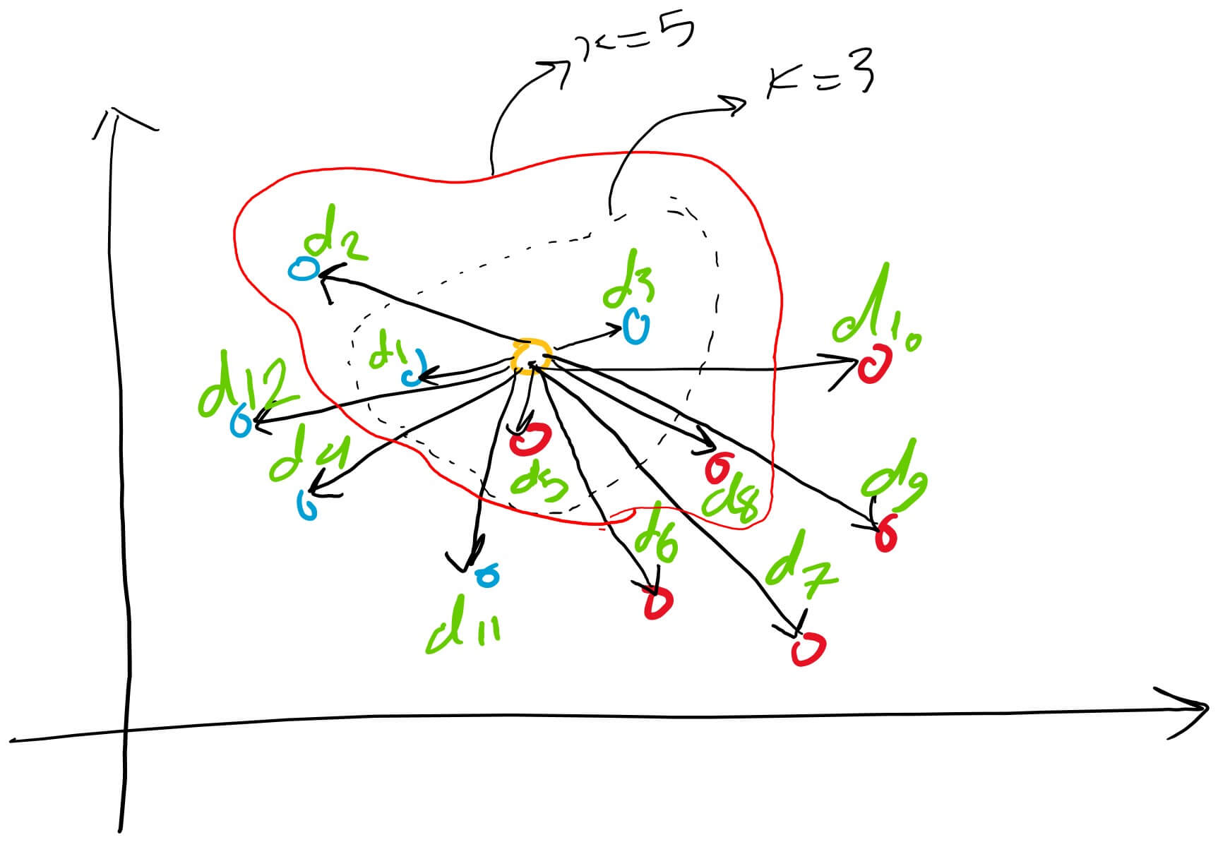
One of the advantages of Random Forest is its versatility, suitable for both classification and regression problems, which dominate current machine learning systems. Here, the performance of Random Forest for `classification` will be explained since classification is sometimes considered a fundamental building block in machine learning. In the image below, two Random Forests created from two trees can be observed.
Random Forest has similar hyperparameters to Decision Trees or Bagging Classifier. Fortunately, there is no need to combine a decision tree with a bagging classifier, and a `Classifier-Class` of the Random Forest can be used. As mentioned earlier, with Random Forest, and, in fact, `Random Forest Regressor,` regression problems can also be addressed.
Random Forest adds an element of randomness to the growth of trees. Instead of searching for the most important features when splitting a `node,` this algorithm looks for the best features among a random set of features. This leads to a high diversity and, ultimately, a better model. Therefore, in Random Forest, only a subset of features is considered by the algorithm to split a node. By adding randomness to the threshold for each feature instead of searching for the best possible threshold, the trees can be made even more random (similar to what a normal decision tree does).
A real-world example of Random Forest
Let’s assume a boy named `Andrew` wants to decide where to travel for a year-long vacation. He requests suggestions from people who know him. Initially, he goes to an old friend and asks about the places he has traveled to in the past and whether he liked those places or not.
Based on this question and answer, the friend suggests several places to Andrew. This approach is common and follows the decision tree algorithm. Andrew’s friend, using his answers, establishes rules to guide his recommendations. After that, Andrew starts asking more and more questions to his friend to receive more recommendations. Similarly, Andrew’s friend asks different questions that can provide recommendations. In the end, Andrew chooses the places that have been recommended to him the most. This overall approach is the essence of the Random Forest algorithm.
Importance of features
Another excellent feature of the Random Forest algorithm is that measuring the relative importance of each feature on the prediction is easy. The Python library ‘scikit-Learn` provides a good tool for this task. This tool measures the importance of a feature by looking at the number of tree nodes that use that feature, and it scales the results, reducing impurity across the forest trees.
This tool automatically calculates and scales the score for each feature after training, so the total sum of all importance scores is equal to 1. Later, a brief explanation of what a `Node` and a `Leaf` are is provided for reference:
In the decision tree, each internal node represents a `test` on features (for example, a coin landing heads or tails), each branch indicates the test output, and each leaf node indicates the category label. The decision is made after calculating all these nodes. A node with no children is considered a `Leaf.`
By examining the importance of features, the user can decide which features may not play a significant role in the decision-making process, either generally or sufficiently. This is crucial because a key rule in machine learning is that the more features there are, the more likely the model is to suffer from `overfitting` or `underfitting.` Below, a table and chart show the importance of 13 features used in a supervised classification project over the course of the Titanic dataset, which is available on Kaggle.
The difference between decision trees and random forests
As mentioned earlier, a random forest is a collection of decision trees. However, there are differences between them. If a dataset with its features and labels is provided as input to the algorithm, it formulates some rules that are used to make predictions. For instance, if a user wants to predict whether a person will click on an online advertisement or not, they can gather ads that the person has clicked on in the past and features describing their decisions. Then, using these, they can predict whether a specific ad will be clicked by a particular person or not.
In comparison, the decision tree algorithm randomly selects observations, builds multiple decision trees based on different features, and then uses the average of the results. Another difference is that a `deep` decision tree may suffer from `overfitting.` Random forests often prevent overfitting by constructing random subtrees from features and building smaller trees from these subtrees, then combining them. It’s worth noting that this solution is not always effective, and the computational process becomes slower with the increasing number of random forests created.
Importance of the hyperparameters
Hyperparameters in random forests are used to enhance the predictive power of the model or speed it up. Next, we will discuss hyperparameters of the random forest function in the sklearn library.
Increasing predictive power
Firstly, there is a hyperparameter called `n_estimators,` representing the number of trees the algorithm creates before reaching maximum votes or averaging predictions. Generally, a higher number of trees improves performance and stabilizes predictions but slows down computations. Another crucial hyperparameter to be discussed is `min_sample_leaf.` This hyperparameter, as implied by its name, specifies the minimum number of leaves needed to split an external node.
Increasing model speed
The `n_jobs` hyperparameter tells the engine how many processors to use. If its value is 1, it can only use one processor. A value of `1` means no limitations. `random_state` makes the model’s output reproducible. When the model has a specific value for random_state, and if hyperparameters and training data similar to it are provided, it always produces similar results. Finally, there is a `oob_score` hyperparameter (also known as oob sampling), which is a method for `out-of-bag validation` in random forests. In this sampling, around one-third of the data is not used for model training and is employed for evaluating its performance. These samples are called `bag samples.` This solution bears resemblance to the `leave-one-out` validation method but is almost computationally free.
Advantages and disadvantages
As mentioned earlier, one of the advantages of a random forest is its versatility for both regression and classification, providing a suitable solution for observing the relative importance assigned to input features. The random forest algorithm is very useful and easy to use due to its default hyperparameters often yielding good predictive results. Additionally, its number of hyperparameters is not high, and they are easy to understand. One of the significant challenges in machine learning is overfitting, but often, this problem does not occur as easily for the random forest classifier as for others. The main limitation of the random forest is that a large number of trees can make the algorithm slow and inefficient for real-world predictions.
In general, training these algorithms is quick, but predicting after the model is trained may become slightly slower. More accurate predictions require more trees, leading to a slower model. In most real-world applications, the random forest algorithm performs fast enough, but there may be conditions where runtime performance is crucial, and other approaches are preferred. However, it’s essential to note that the random forest is a predictive modeling tool rather than a descriptive tool. This means that if the user seeks a descriptive presentation of their data, other approaches are preferred.
Some application areas
The random forest algorithm is used in various fields such as banking, stock markets, medicine, and e-commerce. In banking, it is used to identify customers who use banking services more than others and repay their debts on time. This algorithm is also utilized to detect fraudulent customers planning to defraud the bank.
In financial matters, the random forest is employed to predict stock behavior in the future. In the medical field, this algorithm is used to identify the correct combination of components and analyze a patient’s medical history to diagnose their illness. Finally, in e-commerce, the random forest is used to determine whether customers liked a product or not.
Summary
The random forest algorithm is a good tool for training in the early stages of model development to evaluate its performance. Building a `bad` random forest due to the simplicity of this algorithm is practically more challenging than constructing a good model. Also, if there is a need to develop a model in a shorter timeframe, this algorithm is considered a good option. Moreover, it provides a good index of the importance given to features. Breaking the random forest algorithm in terms of performance is also a difficult task. While it’s possible to find a model like a `neural network` that performs better, these cases likely require more development time. In general, the random forest is often a fast, simple, and flexible tool with its own limitations.
