SQL Tutorial in Two Hours: A Beginner’s Guide

In today’s world, data is everywhere, and its management has become a critical skill in various industries. Structured Query Language (SQL) is a programming language used to manage and manipulate data stored in relational databases. SQL is a vital tool in the data industry, and its demand is on the rise. In this article, we will provide a comprehensive overview of SQL and guide you through the process of mastering the basics in just two hours.

Introduction to SQL Syntax

In this section, we will dive into the practical application of SQL by exploring how to write queries to extract data from a relational database. In Subsection 2.1, we will provide an introduction to SQL syntax and cover the basic structure of a SQL query. We will explain the purpose of keywords such as SELECT, FROM, and WHERE, and show how they can be combined to filter and sort data. We will also cover some basic functions and operators that can be used in SQL, such as COUNT, MAX, MIN, and LIKE. By the end of this subsection, you will have a basic understanding of SQL syntax and be able to write simple queries to extract data from a database.

Let’s provide an example to better understand how to use SQL for a table and manipulate it. We can consider the following table of employees which we have generated randomly. I will explain how you can generate it, but alternatively, you can download the ‘db’ file of this table here and import it into your SQL software.

ID	Name	Age	Gender	Occupation	Income
1	Alice	28	F	Engineer	80000
2	Bob	35	M	Manager	100000
3	Charlie	42	M	Accountant	90000
4	Dana	25	F	Designer	60000
5	Evan	31	M	Programmer	85000
6	Fiona	29	F	HR Specialist	65000
7	George	37	M	Salesperson	75000
8	Holly	26	F	Marketer	70000
9	Ian	33	M	Consultant	95000
10	Jane	24	F	Analyst	65000
11	Karen	28	F	Engineer	82000
12	Larry	35	M	Manager	105000
13	Mike	39	M	Accountant	92000
14	Nancy	27	F	Designer	61000
15	Olivia	32	F	Programmer	87000
16	Peter	30	M	HR Specialist	66000
17	Quinn	38	M	Salesperson	78000
18	Rachel	29	F	Marketer	71000
19	Sam	34	M	Consultant	97000
20	Tom	23	M	Analyst	63000
21	Uma	26	F	Engineer	84000
22	Victor	36	M	Manager	102000
23	Wendy	40	F	Accountant	94000
24	Xander	28	M	Designer	62000
25	Yara	33	F	Programmer	88000
26	Zach	31	M	HR Specialist	67000
27	Ava	39	F	Salesperson	76000
28	Ben	25	M	Marketer	69000
29	Claire	34	F	Consultant	96000
30	Dylan	22	M	Analyst	64000
31	Emily	27	F	Engineer	83000
32	Felix	35	M	Manager	101000

Once you open the file by selecting ‘File’ and then ‘Open Database’, the table will be added to your database, as shown in the figure below, and you can begin working with it.

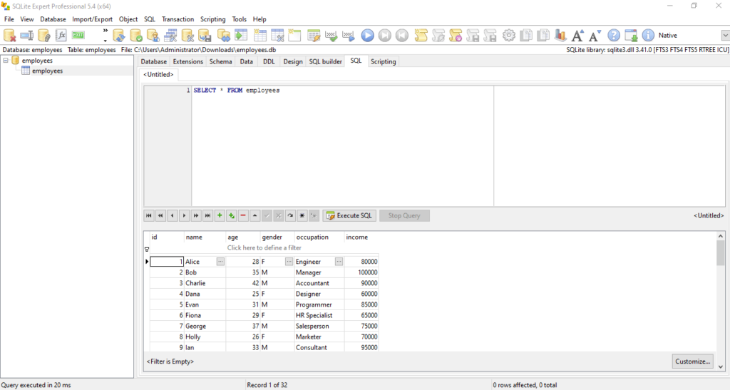
Here are some basic commands to read the table and its columns or rows. In the figure above, we have entered the following line of code to read the entire table:

SELECT * FROM employees

When you put an asterisk (*) after SELECT, it reads all the columns in the table. It does not matter if you write SELECT or select; however, note that SQL software is case-sensitive to the characters in your table. While it does not care about the case of its built-in commands like SELECT/select, it considers ‘Age’ and ‘age’ to be two distinct names.

• Reading columns

To read every column of the table, you can write its name instead of the asterisk symbol. For example, you can use the following command to display every column in the ’employees’ table:

SELECT age FROM employees

If you would like to see more than one specific column, you can separate the names with commas, as follows:

SELECT id, name, age FROM employees

By doing this, SQL will return only the specified columns in the result set, which can help to make your queries more efficient.

• Renaming Columns in SQL

When you’re importing columns and need to assign them new names to differentiate them from the original data, you can use the ‘AS (new name)’ clause immediately after specifying the column name. In the example below, we import the ‘income’ column and rename it as ‘Salary’:

 SELECT income AS Salary FROM employees 

For multiple columns, simply separate them using commas (,). In the following example, we keep the name of the ‘age’ column unchanged but rename ‘income’ and ‘gender’ as ‘Salary’ and ‘Sex’, respectively:

 SELECT age, gender AS Sex, income AS Salary FROM employees 

Note that when renaming a column with a multi-word name, enclose the new name in double quotation marks (“”):

 

 SELECT age AS "years after born" FROM employees 

 

Filtering and Sorting Data

In the second part, we will explore how to filter and sort data using SQL queries. We will cover the various ways to filter data based on specific conditions using the WHERE clause and logical operators such as AND, OR, and NOT. We will also show how to sort data using the ORDER BY clause and how to control the direction of the sorting using ASC and DESC keywords. We will also discuss how to limit the number of results returned by a query using the LIMIT and OFFSET clauses. Additionally, we will cover some common data types used in SQL, such as numbers, strings, and dates, and how to compare and manipulate them in queries. By the end of this subsection, you will have a solid understanding of how to filter and sort data using SQL queries and be able to write more complex queries to extract data from a database.

• Sorting Data

After importing the columns, you can use the ORDER BY clause to sort the data. The examples below illustrate sorting by the ‘name’ column with and without renaming ‘income’ to ‘salary’ before sorting:

SELECT name, income FROM employees ORDER BY name
SELECT name, income AS Salary FROM employees ORDER BY name

You can also sort data by quantitative variables. Here, we sort by the ‘Salary’ (formerly ‘income’) column:

SELECT name, income AS Salary FROM employees ORDER BY Salary
SELECT name, income AS Salary FROM employees ORDER BY income

Both of the above queries yield the same result. By default, sorting is ascending. To specify descending order, use the ‘DESC’ keyword; for ascending order, use ‘ASC’:

SELECT name, income AS Salary FROM employees ORDER BY salary DESC
SELECT name, income AS Salary FROM employees ORDER BY salary ASC

• Filtering Data Using the “WHERE” Clause in SQL

Specific value: The WHERE clause is used to find specific data. For strings, use single quotation marks (‘ ‘) around the value; for numbers, they are not needed. For example:

SELECT name, income AS Salary FROM employees WHERE name = 'Dana'
SELECT name, income AS Salary FROM employees WHERE salary = 60000

Note that theWHEREclause takes precedence over the ORDER BY clause. This means clauses that filter data are processed before other clauses. For instance:

 SELECT name, income AS Salary FROM employees WHERE salary > 60000 ORDER BY salary DESC 

Range Queries: Use the ‘BETWEEN’ clause to filter rows within a specific interval. To find employees with incomes between $60000 and $65000:

 SELECT name, income AS Salary FROM employees WHERE salary BETWEEN 60000 AND 65000 

String and Text Manipulation: To search for names containing ‘an’ or ‘ana’, use the ‘LIKE’ clause:

 SELECT name, income AS Salary FROM employees WHERE name LIKE '_an%' 

In the above example, underscore ‘_’ means any character, and ‘%’ means any sequence of characters. To find any four-letter name which characters 2 to 3 are ‘an’, use ‘_an_‘; to find names ending with ‘na’, use ‘%na’:

SELECT name, income AS Salary FROM employees WHERE name LIKE '_an%'
SELECT name, income AS Salary FROM employees WHERE name LIKE '_an_'
SELECT name, income AS Salary FROM employees WHERE name LIKE '%na'

To filter by specific names, use the ‘IN’ clause. For example, to find names ‘Dana’ and ‘Ian’:

 SELECT name, income AS Salary FROM employees WHERE name IN ('Dana', 'Ian') 

Logical Operators: You can apply multiple conditions to filter rows using the ‘AND’ logical operator. To find names ending with ‘na’ and with a salary over $60000:

 SELECT name, income AS Salary FROM employees WHERE name LIKE '%na' AND salary > 60000 

Additionally, you can locate rows in which the name ends with ‘na’ or the salary is greater than 60000.

 SELECT name, income AS Salary FROM employees WHERE name LIKE '%na' OR salary > 60000 

Null Handling: Use the ‘IS NOT NULL’ condition to exclude rows with null values. To retrieve rows where the name is not null:

 SELECT name, income AS Salary FROM employees WHERE name IS NOT NULL 

To identify Null values, you can use the following query:

 SELECT name, income AS Salary FROM employees WHERE name IS NULL 

Limit Clause: The LIMIT clause is used to restrict the number of rows displayed based on their indices, not their values. For example, in the code below, we display the first 50 rows. In the first query, we specify columns “name” and “income,” while in the second query, we use an asterisk (*) to show all columns.

SELECT name, income FROM employees LIMIT 50;
SELECT * FROM employees LIMIT 50;

Keep in mind that the ORDER BY clause takes precedence over the LIMIT clause, and the LIMIT clause takes precedence over OFFSET. Therefore, the correct order should be as shown below:

 SELECT * FROM employees ORDER BY name LIMIT 50 OFFSET 2; 

COUNT Clause: The COUNT clause calculates the number of rows. You can use it with the WHERE clause to specify conditions. In the following examples, we count the total number of rows in the dataset (first query), and then we count the rows where the income falls within the range [60000, 65000], including both bounds (second query).

SELECT COUNT(*) FROM employees;
SELECT COUNT(*) FROM employees WHERE income BETWEEN 60000 AND 65000;

you can count the distinct values in a column using the COUNT(DISTINCT column) function in SQL. Here’s how you can modify your code to count the distinct ages for each name in the “employees” table:

-- Count distinct ages for each name:
SELECT Name, COUNT(distinct Age) FROM employees
GROUP BY Name;

This query will provide you with the count of unique ages for each unique name in the “employees” table. Now, let’s assume you want to count the rows where the income is greater than 60000, the gender is female, and the name ends with ‘e’:

 SELECT COUNT(*) FROM employees WHERE income > 60000 AND gender = 'F' AND name LIKE '%e'; 

 

Creating and Joining Tables

In this part of the tutorial, we will explore how to create and join tables in SQL to extract data from multiple tables in a relational database. We will cover the different types of joins, including INNER JOIN, LEFT JOIN, RIGHT JOIN, and FULL OUTER JOIN, and when to use each type based on the data you want to retrieve. We will also cover how to join tables on multiple columns and how to use aliases to simplify queries. Additionally, we will discuss how to use subqueries to extract data from one table based on data from another table. By the end of this subsection, you will have a solid understanding of how to join tables in SQL and be able to write more complex queries to extract data from a database with multiple related tables.

• Creating an Empty Table

To create a table in SQL Server named “DataHarnessing,” follow this structure. You can define names for the columns; in this example, we’ll use “col1” and “col2.” Specify the column types right after their names.

 CREATE TABLE DataHarnessing(col1 INTEGER, col2 TEXT); 

• INSERT INTO Clause

The above query creates an empty table. To populate it, use the following query to insert rows. The first column must be an integer, and the second must be a string; otherwise, your software will display an error.

 INSERT INTO DataHarnessing VALUES(1, 'Ishmael'); 

• UPDATE SET Clause

The UPDATE clause allows you to modify table values. In the previous example, we changed the value of the first column to 50 (first line). To update multiple columns, separate them with commas (,). In the second line, we updated the name “Ishmael” to “Ishmael Rezaei.”

UPDATE DataHarnessing SET col1 = 50;
UPDATE DataHarnessing SET col1 = 50, col2 = 'Ishmael Rezaei';

In the INSERT and UPDATE clauses, you don’t necessarily need to enter values for all cells; you can leave them as Null or empty cells. To leave a cell empty, use ”. Empty cells are distinct from Null cells.

INSERT INTO DataHarnessing VALUES(2, Null);
INSERT INTO DataHarnessing VALUES(2, '');

When you have multiple rows and use the UPDATE clause, it changes all values in the column. To avoid this, specify the rows you want to update using the WHERE clause. In the following query, we update rows in the first column where the names are “Ishmael Rezaei.”

 UPDATE DataHarnessing SET col1 = 4 WHERE col2 = 'Ishmael Rezaei'; 

Consider another example: we inserted two rows with NULL names and the value 3. Now, we update the Null values with the name “Peg.”

INSERT INTO DataHarnessing VALUES (3, Null);
INSERT INTO DataHarnessing VALUES (3, Null);
UPDATE DataHarnessing SET col2 = 'Peg' WHERE col1 = 3;

• DELETE FROM Clause

The DELETE FROM clause is used to remove a row from a table. Specify the row you want to delete. Here’s an example of how to delete the first row with values 50 and “Ishmael Rezaei” in columns col1 and col2 separately.

 DELETE FROM DataHarnessing WHERE col1 = 50; 

You can use other filtering clauses that come with the WHERE clause. Note that the DELETE clause deletes rows across all columns. If you want to delete values for specific columns, use Null or ”.

• Deleting a Table with DROP Clause

Assuming the table “DataHarnessing” already exists, use the following query to drop it.

 DROP TABLE DataHarnessing; 

If “DataHarnessing” doesn’t exist, the software will display an error. To avoid this, use the following query.

 DROP TABLE IF EXISTS DataHarnessing; 

Adding a Column:

To add a column in SQL, you can use the following syntax:

 ALTER TABLE dataharnessing 
ADD col4 TEXT;

If you need to create an “id” column that auto-populates when adding rows, you can use this code (note that this may work on SQLite databases):

 DROP TABLE IF EXISTS dataharnessing;
CREATE TABLE dataharnessing (
id INTEGER PRIMARY KEY,
col1 TEXT NOT NULL,
col2 TEXT,
col3 TEXT
);

INSERT INTO dataharnessing (col1, col2, col3) VALUES ('a', 'c', 'c');
INSERT INTO dataharnessing (col1, col2, col3) VALUES ('a', 'c', 'c');
INSERT INTO dataharnessing (col1, col2, col3) VALUES ('a', 'c', 'c');

SELECT * FROM dataharnessing;

ALTER TABLE dataharnessing 
ADD col4 TEXT DEFAULT 'Ali';

SELECT * FROM dataharnessing;

 

Selecting Unique Rows:

To select unique rows for columns “name” and “age,” use the following SQL query:

SELECT DISTINCT name, age 
FROM employees;

To select distinct rows considering all columns:

SELECT DISTINCT * 
FROM employees;

 

Ordering by Multiple Columns:

You can order rows by multiple columns using SQL. For example, to order by “name” in ascending (ASC) order and “age” in descending (DESC) order:

SELECT * 
FROM employees 
ORDER BY name ASC, age DESC;

Conditional Statements:

You can use conditional statements in SQL to define conditions. For example:

 SELECT 
CASE WHEN age > 20 THEN 'true' ELSE 'false' END AS boolA
FROM employees;

SELECT 
CASE age WHEN 25 THEN 'true' ELSE 'false' END AS boolB
FROM employees;

-- For multiple conditions
SELECT 
CASE WHEN age > 20 THEN 'true' ELSE 'false' END AS boolA,
CASE age WHEN 25 THEN 'true' ELSE 'false' END AS boolB
FROM employees;

 

Joining Tables:

To join two tables, for instance, “TableA” and “TableB” on the “Name” column:

 SELECT l.Name, l.Age, r.Name, r.Job 
FROM TableA AS l 
JOIN TableB AS r 
ON l.Name = r.Name;

Renaming Columns:

If you have two columns with the same name after joining tables, you can rename them using the AS keyword:

SELECT l.Name AS Name_l, l.Age, r.Name AS Name_r, r.Job 
FROM TableA AS l 
JOIN TableB AS r 
ON l.Name = r.Name;

Joining Multiple Tables:

To join more than two tables, you can extend the join as needed:

 drop table if exists TableA;
drop table if exists TableB;
drop table if exists TableC;
create table TableA(Name text, Age integer, Income integer);
insert into TableA values('Bob', 32, 80000);
insert into TableA values('Mary', 45, 70000);
insert into TableA values('Hana', 18, 45000);
create table TableB(Name text, Job text);
insert into TableB values('Mary', 'Industrial Engineer');
insert into TableB values('Ishmael', 'Data Scientist');
create table TableC(Id integer primary key, Name text, Education text);
insert into TableC (Name, Education) values('Mary', 'Master');
insert into TableC (Name, Education) values('Ishmael', 'PhD');
insert into TableC (Name, Education) values('Pitter', 'Master');
SELECT l.Name, l.Age, m.Job, r.Education, r.Name 
FROM TableA AS l 
JOIN TableB AS m 
ON l.Name = m.Name 
JOIN TableC AS r 
ON m.Name = r.Name 
ORDER BY l.Name, l.Age;

String Operations:

• To find the length of a string:

SELECT name, age, LENGTH(name) AS 'name length' 
FROM employees;

• To select a part of a string using SUBSTR: It requires giving the name of a column, location of the starting point, and the number of characters, respectively.

SELECT SUBSTR(name, 1, 1) AS 'first char' 
FROM employees;

• To remove spaces in strings using TRIM, LTRIM, and RTRIM:

SELECT TRIM(' string... ',);
SELECT LTRIM(' string... ',);
SELECT LTRIM(' string... ',);
SELECT TRIM('------string... ...---- ', '-');
SELECT LTRIM('------string... ...---- ', '-');
SELECT RTRIM('------string... ...---- ', '-');

• Changing letter case with LOWER and UPPER:

SELECT LOWER('Bob');
SELECT UPPER('bob');

Type

You can determine the type of the inputs using the TYPEOF function as shown below. However, there are some points that need to be considered. Most importantly, you should consult the documentation for your database system since these syntaxes may not make sense for every system.

 SELECT typeof(1);
SELECT typeof('DataHarnessing');
SELECT typeof('Data' + 'Harnessing');

 

 

The three lines return an integer, text, and interestingly, an integer. This is because in SQLite, when you add two text values together, it returns an integer. The type of the inputs is significant because performing algebraic mathematical operations may not yield the same results as it does in other programming languages. For example, if you divide 3 by 2, the result is an integer because both numbers are integers. To obtain a decimal result, you need to specify at least one of the numbers in decimal format.

 SELECT 3/2; -- Returns 1 (integer division)
SELECT 3/2.0; -- Returns 1.5 (decimal division) 

 

Rounding:

You can round numbers using the ROUND function. If you want to round to an integer, you can use either of the following syntaxes:

 SELECT ROUND(34.37432);
SELECT ROUND(34.37432, 0);

If you want to round to three decimal points, you can use:

 SELECT ROUND(34.37432, 3);

Date and Time Functions:

SQLite provides a variety of functions for working with date and time. You can use these functions to retrieve and manipulate date and time information within your database. Here are some examples of how to use these functions:

 -- Get the current datetime
SELECT datetime('now');

-- Get the current date
SELECT date('now');

-- Get the current time
SELECT time('now');

-- Calculate datetime in the future (e.g., 2 years from now)
SELECT datetime('now', '+2 years');

-- Calculate datetime in the past (e.g., 2 years ago)
SELECT datetime('now', '-2 years');

-- Perform detailed datetime calculations
SELECT datetime('now', '+2 hours', '+10 minutes', '+21 days', '+2 years');

SQLite is flexible in handling date and time operations, allowing you to tailor your queries to your specific needs.

Grouping Data:

Data grouping is a crucial aspect of database management, especially when you want to summarize or analyze data efficiently. SQLite provides the GROUP BY clause for this purpose. Let’s say we have an “employees” table, and we want to count the names and group them by the “Age” column:

 SELECT Name, COUNT(*) FROM employees
GROUP BY Age;

Additionally, when you need to join tables and perform data grouping simultaneously, SQLite offers the ability to use multiple WHERE clauses or a HAVING clause, which serves a similar purpose as WHERE in this context. Here’s an example:

 drop table if exists TableA;
drop table if exists TableB;
drop table if exists TableC;
create table TableA(Name text, Age integer, Income integer);
insert into TableA values('Bob', 32, 80000);
insert into TableA values('Mary', 45, 70000);
insert into TableA values('Mary', 42, 70000);
insert into TableA values('Mary', 23, 70000);
insert into TableA values('Mary', 42, 70000);
insert into TableA values('Mary', 23, 70000);
insert into TableA values('Mary', 25, 70000);
insert into TableA values('Mary', 25, 70000);
insert into TableA values('Hana', 18, 45000);
create table TableB(Name text, Job text);
insert into TableB values('Mary', 'Industrial Engineer');
insert into TableB values('Ishmael', 'Data Scientist');
create table TableC(Id integer primary key, Name text, Education text);
insert into TableC (Name, Education) values('Mary', 'Master');
insert into TableC (Name, Education) values('Mary', 'Bachelor');
insert into TableC (Name, Education) values('Ishmael', 'PhD');
insert into TableC (Name, Education) values('Pitter', 'Master');
SELECT l.Name, l.Age, m.Job, r.Education, r.Name
FROM TableA AS l 
JOIN TableB AS m 
ON l.Name = m.Name
JOIN TableC AS r 
ON m.Name = r.Name
where r.Education != 'Master'
group by l.Age
having Age != 25
ORDER BY l.Name, l.Age;

In this example, we’re joining three tables and grouping the results based on the “Age” column, excluding entries where “Education” is “Master” and filtering out records with an “Age” of 25.

you can use various aggregate functions like avg, max, min, and sum with the GROUP BY clause to analyze your data in different ways. Here’s how you can modify your code to include these functions:

 -- Group data and calculate average age:
SELECT Name, avg(Age) FROM employees
GROUP BY Name;
-- Group data and calculate maximum age:
SELECT Name, max(Age) FROM employees
GROUP BY Name;
-- Group data and calculate minimum age:
SELECT Name, min(Age) FROM employees
GROUP BY Name;
-- Group data and calculate the sum of ages:
SELECT Name, sum(Age) FROM employees
GROUP BY Name; 

With these SQL queries, you can analyze your employee data by calculating the average, maximum, minimum, and sum of ages for each unique name in the “employees” table.

TRANSACTION:

A ‘TRANSACTION’ is used to execute multiple SQL statements simultaneously and in a mutually exclusive manner. If one statement fails, all the subsequent statements within the transaction will also fail. During a transaction, if you realize that a mistake has been made, you can use the ‘ROLLBACK’ command to undo the previous statements. Here is an example:

 BEGIN TRANSACTION;
-- Your update statement(s) here
UPDATE TableA SET Age = Age - 1 WHERE Age = 45;

COMMI;

 BEGIN TRANSACTION;
-- Your update statement(s) here
UPDATE TableA SET Age = Age - 1 WHERE Age = 45;
ROLLBACK; -- Use ROLLBACK to cancel the transaction and revert changes

You have the option to either use ‘END TRANSACTION’ or ‘COMMIT’ to conclude the transaction. It’s important to note that each line in SQL statements should end with a semicolon, including at the beginning and end.

You have the option to either use END TRANSACTION or COMMIT to conclude the transaction. It’s important to note that each line in SQL statements should end with a semicolon, including at the beginning and end.

Trigger:

Suppose you have a table called “Orders” with columns “OrderID,” “CustomerName,” and “OrderDate,” and you want to update the “OrderDate” column with the current timestamp whenever a new order is inserted.

 -- Create a table

CREATE TABLE Orders (

OrderID INTEGER PRIMARY KEY,

CustomerName TEXT,

OrderDate TEXT

);

-- Create a trigger to update OrderDate when a new row is inserted

CREATE TRIGGER UpdateOrderDate

AFTER INSERT ON Orders

BEGIN

UPDATE Orders

SET OrderDate = DATETIME('now')

WHERE OrderID = NEW.OrderID;

END;

-- Insert a new row into the Orders table

INSERT INTO Orders (CustomerName) VALUES ('John Doe');

-- Query the Orders table to see the result

SELECT * FROM Orders;

 

We create a table called “Orders” with columns “OrderID,” “CustomerName,” and “OrderDate.” We create a trigger named “UpdateOrderDate” that activates after an insert operation on the “Orders” table. Inside the trigger, we use the UPDATE statement to set the “OrderDate” column to the current timestamp using DATETIME(‘now’) for the newly inserted row, identified by NEW.OrderID. We then insert a new row into the “Orders” table with just the “CustomerName” column filled. When we query the “Orders” table, we’ll see that the “OrderDate” column has been automatically updated with the current timestamp for the newly inserted row, thanks to the trigger.

Subselect:

You can combine two ‘SELECT’ statements using a subquery like this:

 select NA from (select Name as NA from TableA) 

In this example, we create a subquery (also known as a subselect) by selecting the ‘Name’ column from ‘TableA’ and aliasing it as ‘NA.’